If you cut across all the tiresome hype and snake oil marketing that surrounds the AI / Machine Learning field you can find valuable techniques that can provide value to software projects. This is especially true for those that revolve around data sharing and publication like data catalogs. They are (generally) well-structured repositories of (hopefully) publicly available data described by (one would hope) comprehensive dataset metadata, all good ingredients to apply to ML processes. There have been promising attempts in CKAN to integrate with LLM-powered chatbots, and things like automatic dataset classification or semantic search look like they could add value with relatively low effort.
To learn more and focus on one particular feature, I’ve been recently exploring the use of embeddings to find similar datasets in large CKAN instances. I’ve split the writing in two posts, this one gives a very high level introduction to what embeddings are, and a second part touches on the actual implementation of a CKAN extension. If you are familiar with embeddings you can skip to part 2:
Part 2: Building a CKAN extension that leverages embeddings
| Disclaimer |
|---|
| The following is meant to be a gentle introduction to folks that are not familiar with Machine Learning concepts and just need a high level overview to get started. I’m sure that I’m missing stuff and oversimplifying a lot of things but keep in mind the intended audience. But of course if you notice an error please let me know! |
What are embeddings?
There are long mathematical explanations to what embeddings are and how are they computed but for our purposes let’s say that embeddings are a way of encoding complex information like texts, images or data into a standard numerical representation, a vector (a fancy name for a list of numbers). The important bit is that this numerical representation captures the semantic meaning of the original input, at least according to the underlying model used to create the embeddings.
This makes easy for computers to compare embeddings between them, and calculate which ones are closer to others, that is which original objects are more similar between them.
Let’s see an example. Here are the simplified embeddings of some pieces of text using Sentence Transformers’s all-MiniLM-L6-v2 model (All embeddings computed using the same model have the same dimensions, i.e. the list of numbers has the same size):
| Text | Embedding (5 first dimensions) |
|---|---|
| A dog with a blue hat | [ -0.01296314, 0.00495872, 0.06955151, 0.05257371, 0.0787459, …] |
| A cat with a blue hat | [ 0.04728317, 0.03822584, 0.05235671, 0.0423677, 0.01458137, …] |
| A fish with a blue hat | [ -0.0333364 , 0.07279811, -0.00606286, -0.01582586, 0.03766956, …] |
| Stately, plump Buck Mulligan came from the stairhead | [ -0.05418522, 0.01471444, 0.01173631, 0.02672934, 0.0138136, …] |
You can use a different model to compute the embeddings, for instance OpenAI’s text-embedding-ada-002. In this case the embeddings would have 1536 dimensions instead of 384.
Comparing things with embeddings
Now that we have our pieces of information encoded as embeddings we can use one of the different available algorithms to find out which embeddings are more similar to others (or how close are the locations defined by each embedding in a multi-dimensional space if you prefer).
For comparing word-based sentence embeddings a common technique is to compute the cosine similarity between them (all commonly used ML libraries will be able to use this and other algorithms available, I used SentenceTransformers). Let’s see what the cosine similarity values are for the texts above (the closer the cosine similarity value is to 1, the closer the two sentences are according to the model):
| A dog with a blue hat | A cat with a blue hat | A fish with a blue hat | Stately, plump Buck Mulligan came from the stairhead | |
|---|---|---|---|---|
| A dog with a blue hat | 1 | 0.7371 | 0.6691 | 0.1455 |
| A cat with a blue hat | 1 | 0.6176 | 0.0306 | |
| A fish with a blue hat | 1 | 0.0900 | ||
| Stately, plump Buck Mulligan came from the stairhead | 1 |
We can clearly see that animals wearing a blue hat are closer together, and that cats are closer to dogs than fishes. And of course all three sentences are very different from James Joyce’s Ulysses opening words.
As I mentioned earlier, embeddings are not limited to text inputs. We can use models that have been trained on image/text pairs, which can understand both image and text inputs (these are called multimodal models). This time, we will find the cosine similarity between the embeddings of an image and the same texts we used before. To do so we will use a multimodal model, OpenAI’s CLIP. SentenceTransformers provides a handy wrapper to interact with it:
| A dog with a blue hat | A cat with a blue hat | A fish with a blue hat | Stately, plump Buck Mulligan came from the stairhead | |
|---|---|---|---|---|
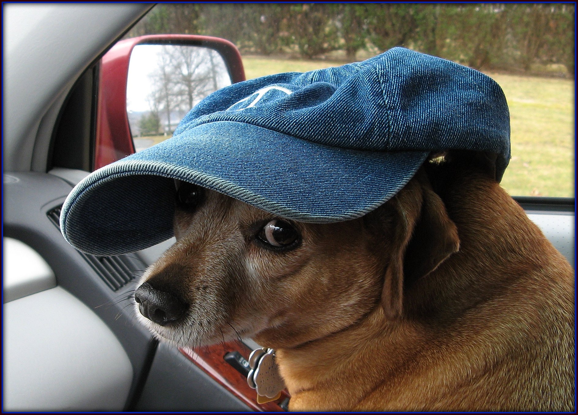 Pic courtesy of Tony Fischer on Flickr |
0.3288 | 0.2703 | 0.2589 | 0.2202 |
Again, the closer embedding to the image one was the text describing it, followed by the other hat-wearing animal sentences.
A word of caution
The ability to get semantic similarity between different texts or other inputs feels like magic and it’s tempting to dive straight into integrating it in existing systems, but it is important to remember that the original embeddings were computed based on a specific model. This model was in turn trained on a specific set of data (a really big set!), so the representation of any input data (and their similarity to other data inputs) will reflect any existing biases present in the original data the model was trained on.
See for instance the following similarities:
| a white person | a young black man | a woman | a black person | an immigrant | |
|---|---|---|---|---|---|
| poor people | 0.1631 | 0.1876 | 0.0899 | 0.2031 | 0.2435 |
| a nice person | 0.4470 | 0.3054 | 0.4118 | 0.4620 | 0.3576 |
| a thief | 0.3151 | 0.2752 | 0.2781 | 0.4007 | 0.3701 |
Just to be clear, I’m sure that there are a lot of flaws with this quick test and I can’t claim to understand the relevance of the exact values returned and the differences between them. But it’s telling that in almost all cases texts describing minorities are closer to texts describing negative qualities.
This doesn’t mean that we should not use embeddings, but we need to think in the way in which they will integrate in our application and identify potential ways in which these biases could affect the intended feature.
Leveraging this in our application
The relatively simple technique we have described has many diverse uses. Common ones include content suggestions, recommendation systems, semantic search, image search, etc but embeddings can be applied to many different kinds of data like user profiles, audio samples, time series etc.
For our original data catalogs target we’ll explore applying embeddings to implement two useful features:
-
Finding similar datasets: this is the most straightforward one, given a particular dataset of interest, which are the most similar ones that might be also of interest?
-
Semantic search: let’s see if we can enrich the traditional text-based search that powers most portals with a semantic one to increase discoverability.
In the next post in this series I’ll go into detail on how to build a CKAN extension that implements these two features.